note5_policy_based

policy gradient

• On-policy: The agent learned and the agent interacting with the environment is the same.

• Off-policy: The agent learned and the agent interacting with the environment is different

• paper

  • policy_gradient
  • dpg
  • ddpg

• 优势

  • 连续动作
  • 随机策略
• 参考
  • Pong from Pixels-en
  • Pong from Pixels-ch

function approximation

在value_based方法中，由参数$w$对价值函数进行近似表示： $$\hat{q}(s,a,w)\approx q_{\pi}(s,a)$$ 在policy_based方法中，策略$\pi$被描述为一个包含参数$\theta$的函数，即最优策略是由以状态作为输入的网络输出的概率值来决定的： $$\pi_\theta(s,a)=P(a|s,\theta)\approx\pi(a|s)$$

If the action space is discrete and not too large, then a natural and common kind of parameterization is to form parameterized numerical preferences $h(s,a,\theta)\in R$ for each state–action pair. The actions with the highest preferences in each state are given the highest probabilities of being selected, for example, according to an exponential softmax distribution: $$\pi(a|s,\theta)=\frac{e^{h(s,a,\theta)}}{\sum_b e^{h(s,b,\theta)}}$$ The action preferences $h$ themselves can be parameterized arbitrarily, by deep neural network or just linear, $h(s,a,\theta)=\theta^Tx(s,a)$

the advantage of parameterizing policies according to the softmax in action preferences:
- the approximate policy can approach a deterministic policy - enables the selection of actions with arbitrary probabilities

softmax policy

$$\pi(a|s,\theta)=\frac{e^{h(s,a,\theta)}}{\sum_b e^{h(s,b,\theta)}} \\ \pi(a|s,\theta) \propto e^{h(s,a,\theta)} \\ \nabla_{\theta} \log \pi_{\theta}(s, a)=h(s, a)-\mathbb{E}_{\pi_{\theta}}[h(s, \cdot)]$$

objective

$J(\theta)$: performance measure

在这里神经网络的更新不是依靠误差，而是依靠奖励。梯度上升法最大化目标函数。奖励值越大则占越大的比重。

1. start value: 在一个完整的序列下，以初始状态的累计奖励值来衡量策略的优势. $V_{\pi_\theta}$ is the true value for $\pi_\theta$, the policy determined by $\theta$. In this discussion the discounting rate $\gamma$ is not included. $$J_1(\theta)=V_{\pi_\theta}(s_1)=E_{\pi_\theta}[v_1]$$
2. average reward: 在连续环境条件下，不存在某个初始状态。把个体在某时data_path刻下的状态看成各个状态概率分布，则把每一时刻得到的奖励按各状态的概率分布求和, $d_{\pi\theta}$是在某一策略下的s的概率分布： $$J_{avV}(\theta)=\sum_sd_{\pi_\theta}V_{\pi_\theta}(s)$$
3. average reward per time-step: 每一时间步长下的平均奖励： $$J_{avR}(\theta)=\sum_sd_{\pi_\theta}(s)\sum_a\pi_\theta(s,a)R^a_s$$

policy gradient theorem

$$\bigtriangledown J(\theta)\propto \sum_s d_{\pi_\theta}(s)\sum_{a}q_\pi(s,a)\bigtriangledown \pi(a|s,\theta)$$

梯度的中间变形：

$$\begin{aligned} \nabla_{\theta} \boldsymbol{\pi}_{\theta}(\mathbf{s}, \mathbf{a}) &=\frac{\boldsymbol{\pi}_{\theta}(\mathbf{s}, \mathbf{a})}{\boldsymbol{\pi}_{\theta}(\mathbf{s}, \mathbf{a})} \nabla_{\theta} \boldsymbol{\pi}_{\theta}(\mathbf{s}, \mathbf{a}) \\ &=\boldsymbol{\pi}_{\theta}(\mathbf{s}, \mathbf{a}) \frac{\nabla_{\theta} \boldsymbol{\pi}_{\theta}(\mathbf{s}, \mathbf{a})}{\boldsymbol{\pi}_{\theta}(\mathbf{s}, \mathbf{a})} \\ &=\boldsymbol{\pi}_{\theta}(\mathbf{S}, \mathrm{a}) \nabla_{\theta} \log \boldsymbol{\pi}_{\theta}(\mathbf{s}, \mathbf{a}) \end{aligned}$$

假设目标函数如下所示，$x\sim p(x|\theta)$表示变量x服从以$\theta$为参数的$p(x|\theta)$分布，而我们的目地是求$f(x)$在概率分布$p(x|\theta)$下的期望。若$f(x)$表示reward，则在策略梯度求解中的目地是通过改变$\theta$的值，来改变x的分布，从而使得$J(\theta)$最大化。 $$J(\theta)=E_{x\sim p(x|\theta)}(f(x))$$ 目标函数的梯度求解： $$\begin{align} \bigtriangledown E_{x\sim p(x|\theta)}(f(x))&=\bigtriangledown_\theta\sum_xp(x|\theta)f(x)\\ &=\sum_x \bigtriangledown_\theta p(x|\theta)f(x)\\ &=\sum_x p(x|\theta) \frac{\bigtriangledown_\theta p(x|\theta)}{p(x|\theta)}f(x) \\ &=\sum_x p(x|\theta) \bigtriangledown_\theta \log p(x|\theta)f(x) \\ &=E(f(x)\bigtriangledown_\theta \log p(x|\theta)) \end{align}$$

reinforce

基于整个回合数据的方法，称为reinforce算法。这里基于Monte Carto进行采样。在梯度上升更新过程中，右乘的$v_t$是该动作的奖励值，奖励值的大小影响上升梯度中由该动作所造成的梯度。（让原始策略先跑一轮，若得到正向反馈，增加选择该动作的概率，若得到负向反馈，则减少选择该动作的概率，从而更新策略。以数学的角度来看，反馈即是reward，梯度又乘便得到反馈对梯度的选择作用，参数更新即是在更新策略。）

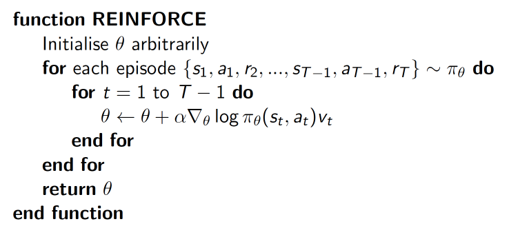
最大化$\log\pi_\theta(s,a)v$等效于最小化-$\log\pi_\theta(s,a)v$，故在tensorflow中的处理可以用交叉熵最小化loss：

neg_log_prob = tf.nn.sparse_softmax_cross_entropy_with_logits(logits=softmax_input_act, labels=tf_acts)
loss = tf.reduce_mean(neg_log_prob *tf_vt)

tips:

1. 对reward做归一化（减去平均值，除以标准差）
2. 引入discount rate. 玩游戏的输赢到最后一步才会给出reward。而在更通用的增强学习设定中我们在每一个时间点都会得到一些回馈$r_t$。一个常用的选择是使用折扣化的回馈$R_t=\sum_{k=0}\gamma^k r_{t+k}$

actor-critic

• 可以单步更新，不再需要完整序列，比传统policy gradient更快
• 难以收敛

learn approximations to both policy and value functions.

• critic: 更新价值函数网络参数
• actor: 更新策略函数网络参数

for each step: 1. initialize $w,\theta,s$ 2. a=$\phi(s)$, $r,s'$=env.step(a) 3. $V(s)=Q(s),V'(s')=Q(s')$ 4. TD error: $\bigtriangledown=R+\gamma V(s')-V(s)$ 5. train network: - w:=w+$\bigtriangledown^2$ - $\theta:=\theta+\bigtriangledown\log \pi_\theta(s,a)\bigtriangledown$

A3C

DDPG: Deep Deterministic Policy Gradient

参考DDQN，actor和critic分别建立两个网络进行更新和矫正。初始化s,由actor网络得出a, 根据env.step(a)得出新的s_和r. 首先根据r更新critic网络，然后根据critic建议的方向(q(s,a))去更新actor网络。

critic的网络更新策略与DDQN类似，但是actor的更新策略看上去很复杂。但是Actor的损失可以简单的理解为得到的反馈Q值越大损失越小，得到的反馈Q值越小损失越大，因此只要对状态估计网络返回的Q值取个负号即可，即： $$J(\theta)=-\frac{1}{m}\sum_{j=1}^m Q(s,a,w)$$

tips: - 对动作增加随机噪音：$A=\pi_theta(S)+N$ - exponential moving average: 网络参数步进复制，$w'=\tau w+(1-\tau)w'$, $\theta=\tau \theta+(1-\tau)\theta'$