note2_rl

Reinforcement Learning

deep rl tutorial in icml 2016

相比与监督学习，强化学习没有训练数据的输出值，但是有奖励值； 相比与无监督学习，除了训练数据还有奖励规则。

• env: environment
• agent: intelligent robot

强化学习八要素：

1. S: state
2. A: action
3. R: reward，个体在$S_t$采取动作$A_t$对应的奖励为$R_{t+1}$
4. $\pi$: policy,策略，即在某一状态下如何选择动作，常以条件概率表示为$\pi(a/s)=P(A_t=a|S_t=s)$，即在状态s时采取动作a的概率
5. v: value, 在策略$\pi$和状态s下，进入下一个状态后的价值，又被称为值函数，表示为$v_\pi(s)$. 事实上值函数代表当前状态的价值，而是否能达到目的还跟未来的状态有关，故当前值函数也跟未来状态的值函数有关。v函数可以理解为是在状态稳定之后的该状态下的最终的结果，而R函数是当前的即时奖励。 $$v_\pi(s)=\mathbf{E}_\pi(R_{t+1}+\gamma R_{t+2}+\cdots| S_t=s)$$
6. $\gamma$: discount rate(reward decay rate), 如果为0，则是贪婪法，即价值只由当前延时奖励决定，如果是1，则所有的后续状态奖励和当前奖励一视同仁。大多数时候，我们会取一个0到1之间的数字，即当前延时奖励的权重比后续奖励的权重大
7. $P^a_{ss'}$: state transition model，在当前状态s采取动作a后转到下一个状态s‘的概率，虽然大部分问题的的状态转化模型为1. P predicts the next state, R predicts the next reward. $$P^a_{ss'}=P[S_{t+1}=s'|S_t=s,A_t=a] \\ R^a_s=E[R_{t+1}|S_t=s,A_t=a]$$
8. $\epsilon$: exploration rate

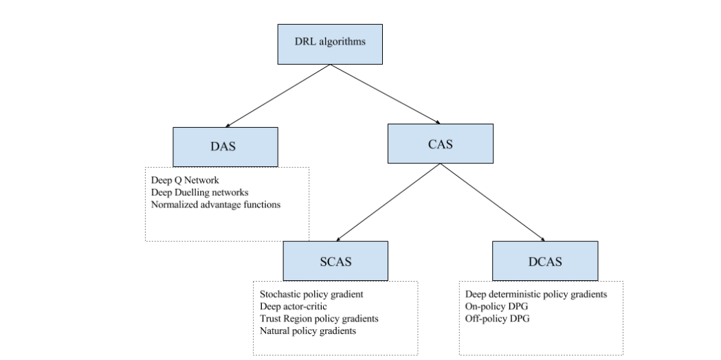
approaches to reinforcement learning: Using deep networks to represent value, policy, model

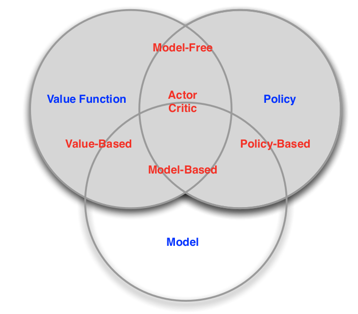
• categorizing 1
  • valued-based
  • policy-based
  • actor critic
    • policy
    • value function
• categorizing 2
  • model free
    • policy and/or value function
  • model based
    • policy and/or value function
    • model

prediction and control

• prediction: evaluate the future
  • given a policy

• control: optimise the future

  • find the best policy

• 预测：给定强化学习的6个要素：状态集S, 动作集A, 模型状态转化概率矩阵P, 即时奖励$r$，衰减因子$\gamma$, 给定策略$\pi$， 求解该策略的状态价值函数$v(\pi)$

• 控制：求解最优的价值函数和策略。给定强化学习的5个要素：状态集S, 动作集A, 模型状态转化概率矩阵P, 即时奖励r，衰减因子$\gamma$, 求解最优的状态价值函数$v_$和最优策略$\pi_$

helpful equation

• 条件边缘概率：$\rho(Z|X)=\sum_Y\rho(Z|X,Y)\rho(Y|X)$
• 条件期望：$E[g(Z)|X]=\sum_Zg(Z)\rho(Z|X)$

Markov Decision Process

The agent’s goal is to maximize the cumulative reward: $$G_t=R_{t+1}+R_{t+2}+\cdots+R_T,\\ \text{T is the terminal step}$$ Discounting reward for a continuous episode: $$G_t=R_{t+1}+\gamma R_{t+2}+\cdots=\sum_{k=0}^\infty \gamma^kR_{t+k+1}$$ If $0<\gamma< 1$, the sum will be finite as $R_{t}$ is bounded. $\gamma+\gamma^2+\cdots+\infty=\frac{1}{1-\gamma}$

• 状态转化模型：$P_{ss'}^a=E(S_{t+1}=s'|S_t=s,A_t=a)$
• policy：$\pi(a/s)=P(A_t=a|S_t=s)$
• state-value function under policy $\pi$：$v_\pi(s)=E(G_t|S_t=s)=E_\pi(R_{t+1}+\gamma R_{t+2}+\cdots| S_t=s)$
• action-value function for policy $\pi$：$q_\pi(s,a)=E(G_t|S_t=s,A_t=a)=E_\pi(R_{t+1}+\gamma R_{t+2}+\cdots| S_t=s,A_t=a)$

价值函数表示该状态下的价值，而动作价值函数是在该状态下可能的各个动作的价值，价值函数是由这些动作价值函数的期望共同构成的。

递推关系:

$$v_\pi(s)=\sum_{a\in A}\pi(a/s)q_\pi(s,a)\\ q_\pi(s,a)=R_{t+1}+\gamma\sum_{s'\in S}P_{ss'}^av_\pi(s')\\ v_\pi(s)=\sum_{a\in A}\pi(a/s)(R_{t+1}+\gamma\sum_{s'\in S}P_{ss'}^av_\pi(s'))\\ q_\pi(s,a)=R_{t+1}+\gamma\sum_{s'\in S}P_{ss'}^a\sum_{a\in A}\pi(a'/s')q_\pi(s',a')$$

最优价值函数： 在局部最优的策略下，状态价值函数应局部最大，动作价值函数应局部最大。

$$v_*(s)=\max_{\pi}v_\pi(s)\\ q_*(s,a)=\max_{\pi}q_\pi(s,a)\\ \pi_*(a/s)= \begin{cases} 0& \text{if } a=\arg \max_{a\in A}q_*(s,a)\\ 1& \text{else} \end{cases}$$

因此值函数便不再是各个值函数的期望，而直接选择最大的值函数。 $$v_*\pi*(s)=\max_a(R_{t+1}+\gamma\sum_{s'\in S}P_{ss'}^av_*(s'))\\ q_*(s,a)=R_{t+1}+\gamma\sum_{s'\in S}P_{ss'}^a\max_{a'}q_*(s',a')$$

ergodic Markov process

Dynamic Programming

Dynamic programming is a method for solving complex problems by breaking them down into subproblems and MDP just satisfy the property. - for prediction - input: MDP$$ and policy $\pi$ - output: value function $v_\pi$ - for control - input: MDP$$ - output: optimal value function $v_$ and optimal policy $\pi_$

$$\begin{align}v_\pi(s)&=\sum_{a\in A}\pi(a/s)(r+\gamma\sum_{s'\in S}P_{ss'}^av_\pi(s')) \\ &=\sum_{a\in A}\pi(a/s)\sum_{s'\in S}P_{ss'}^a(r+\gamma v_\pi(s')) \\ &=\sum_{a\in A}\pi(a/s)\sum_{s',r}p(s',r|s,a)(r+\gamma v_\pi(s')) \end{align}$$

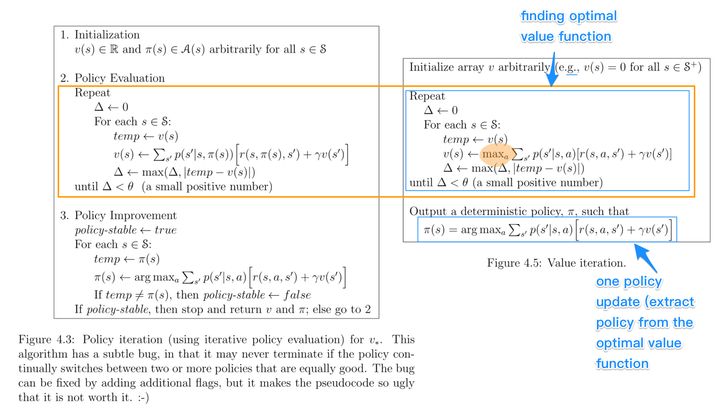
Policy Iteration

策略迭代包括策略估计和策略提升。策略评估过程中根据当前策略迭代使得值函数收敛。提升阶段是根据评估时的值函数更新策略。

1. policy evaluation:

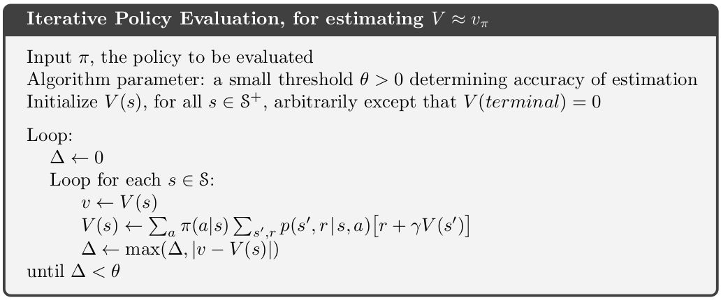
策略已知，通过值函数迭代公式使值函数收敛（$\Delta v=0$）。

1. Policy improvement

improve the policy by acting greedily: $$\pi^*(s)=arg\max_{a\in A}q_\pi(s,a)\\ q_\pi(s,\pi^*(s))=\max_{a\in A}q_\pi(s,a)=v_{\pi^*}(s)\geq q_\pi(s,a)=v_\pi(s)$$ when the iteration stop: $$q_\pi(s,\pi^*(s))=v_{\pi^*}(s)=v_\pi(s)$$ the optimal value funtion and optimal policy are found.

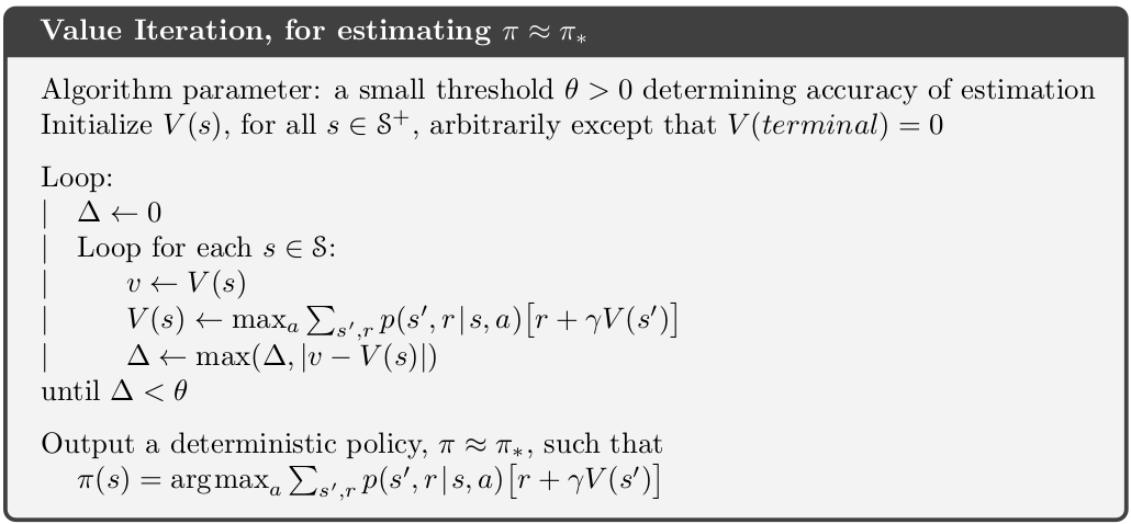
在值函数未知及策略未知的情况下（由于最优策略可完全由最有值函数得出，故值函数未知，则最优策略未知），通过值函数迭代公式使值函数收敛（$\Delta v=0$），收敛后的值函数便是所求的值函数，因此最优策略也可因此而得出。这里的值函数迭代由于没有策略函数，故采用最优值函数迭代公式，即策略是选择局部最大值函数进行迭代。

value iteration

值迭代再每一步值更新的过程中都重新选择策略，减少了迭代次数。值迭代的更新公式其实就是贝尔曼最优公式。

对于预测问题，相当策略已知，通过贝尔曼方程迭代可以求得。而对于控制问题，需要不断更新Q表使其收敛，则最优策略也即得出（最有策略依据最大值函数）。策略迭代：根据探索率更新策略。价值迭代：探索率接近0时，依据值函数更新。

policy-iteration vs value-iteration

• 在Policy Iteration中
  • 第一步 Policy Eval：一直迭代至收敛，获得准确的V(s)
  • 第二步 Policy Improvement：根据准确的V(s)，求解最好的Action
• 对比之下，在Value Iteration中
  • 第一步 "Policy Eval"：迭代只做一步，获得不太准确的V(s)
  • 第二步 "Policy Improvement"：根据不太准确的V(s)，求解最好的Action

这两种迭代过程都需要知道采取该动作后的奖励值是多少。

asynchronous dynamic programming - in-place dtnamic programming

not(two copies of value function): $v_{new}(s)\leftarrow\max{a}(R^a_s+\gamma\sum_{s'\in S}P^a_{ss'}v_{old}(s'))$
but(one copy of value function): $v(s)\leftarrow\max{a}(R^a_s+\gamma\sum_{s'\in S}P^a_{ss'}v(s'))$

• prioritisedd sweeping: use the magnitude of Bellman error to guide state selection $$|\max_{a}(R^a_s+\gamma\sum_{s'\in S}P^a_{ss'}v(s'))-v(s)|$$

• real-time dynamic programming

Monte Carlo Methods

We do not assume complete knowledge of the environment. To sample some complete episodes.

不基于模型的强化学习问题，即状态转化概率未知。

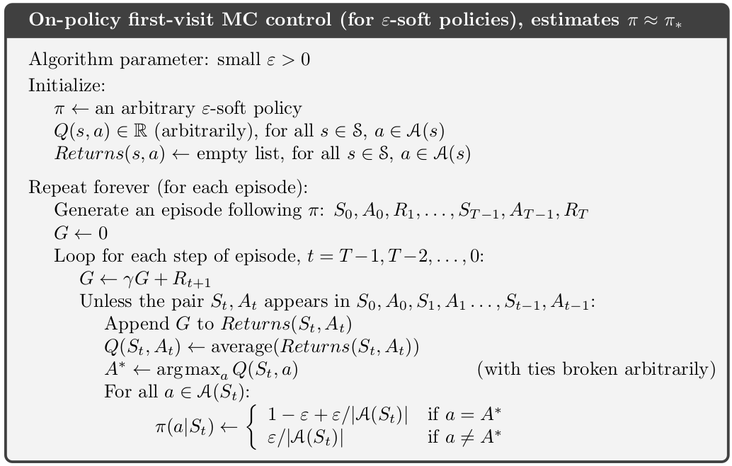
• prediction: $$G_t=R_{t+1}+\gamma R_{t+2}+\cdots \\ v_\pi(s)\approx average(G_t)$$

  • If one state appears many times in one episode:first visit- only consider the first show-up value; every visit- calculate the average
  • incremental mean: $\mu_k=\frac{1}{k}\sum^k_{j=1}=\mu_{k-1}+\frac{1}{k}(x_k-\mu_{k-1})$
  • control: update every step
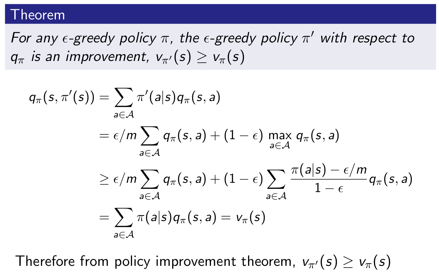
  • greedy policy improvement over $v(s)$ requires model of MDP $$\pi'(s)=arg\max_{a\in A}R^a_s+P^a_{ss'}v(s')$$
  • greedy policy improvement over $q(s,a)$ is model-free $$\pi'(s)=arg\max_{a\in A} q(s,a)$$
  • $\epsilon$ greedy:most of the time they choose an action that has maximal estimated action value, but with probability $\epsilon$ they instead select an action at random. $m=|A(t)|$ is the number of action space dim. $$\pi(a|s)=\left\{ \begin{aligned} = & \epsilon/m+1-\epsilon \quad \text{if } a^*=arg\max Q(s,a) \\ = & \epsilon/m \text{ else} \end{aligned} \right.$$

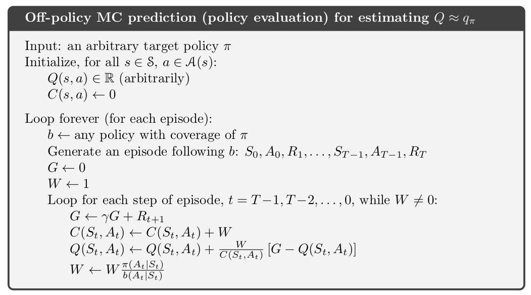
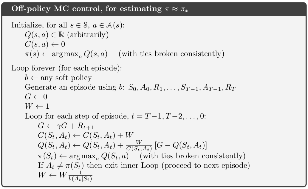
off policy

• on policy:生成样本的policy（value function）跟网络更新参数时使用的policy（value function）相同. 可能会陷入局部最优。
• off policy: 生成样本的policy（value function）跟网络更新参数时使用的policy（value function）不同. Evaluate target policy $\pi(a|s)$ to compute $v_\pi(s)$ or $q_\pi(s,a)$ while following behaviour policy $\mu(a|s)$: ${S_1,A_1,R_1,\cdots,S_T}\sim\mu$

importance sampling: 用一个简单分布去估计服从另一个分布的随机变量的均值

$$\begin{align}E_{X\sim P}[f(x)]&=\sum P(X)f(X) \\ &=\sum Q(X) \frac{P(X)}{Q(X)}f(X) \\ &=E_{X\sim Q} \frac{P(X)}{Q(X)}f(X) \end{align}$$

Use returns generated from $\mu$ to evaluate $\pi$ with weight return $G_t$ according to similarity between policies:

$$G_t^{\pi/\mu}=\frac{\pi(A_t|S_t)\pi(A_{t+1}|S_{t+1})\cdots \pi(A_T|S_T)}{\mu(A_t|S_t)\mu(A_{t+1}|S_{t+1})\cdots \mu(A_T|S_T)} G_t$$ Update value towards corrected return: $$V(S_t)\leftarrow V(S_t)+\alpha(G_t^{\pi/\mu}-V(S_t))$$

Incremental Implementation

Temporal-Difference Learning

learns from incomplete episode

$$G(t)=R_{t+1}+V(S_{t+1})$$ iteration, $\alpha\in [0,1]$: $$V(S_t)=V(S_t)+\alpha(G(t)-V(S_t)) \\ Q(S_t,A_t)=Q(S_t,A_t)+\alpha(G(t)-Q(S_t,A_t))$$

TD($\lambda$)

$$G^\lambda(t)=(1-\lambda)\sum^\infty_{n=1}\lambda^{n-1}G_t^{(n)}$$ $$V(S_t)=V(S_t)+\alpha(G^\lambda(t)-V(S_t)) \\ Q(S_t,A_t)=Q(S_t,A_t)+\alpha(G^\lambda(t)-Q(S_t,A_t))$$

on policy: SARSA

$$Q(S,A)=Q(S,A)+\alpha(R+\gamma Q(S',A')-Q(S,A))$$

off policy: Q learning

$$Q(S,A)=Q(S,A)+\alpha(R+\gamma \max_{a}Q(S',A)-Q(S,A))$$

overview

from 2017-Deep reinforcement learning for robotic manipulation-the state of the art