Gaussian Process Motion Planner (GPMP)

Gaussian Process

ref:

• blog
  • Gaussian-Processes-Regression-Tutorial
  • Gaussians process cartoon
  • Gaussian processes for nonlinear regression lecture
  • gaussian-process-tutorial
• project
  • vizgp
• paper
  • Machine learning cheat sheet
• book
  • GPML

Multivariate Normal Distribution (MVN) Mixtures of Gaussians (MoG)

Gaussian Process Regression

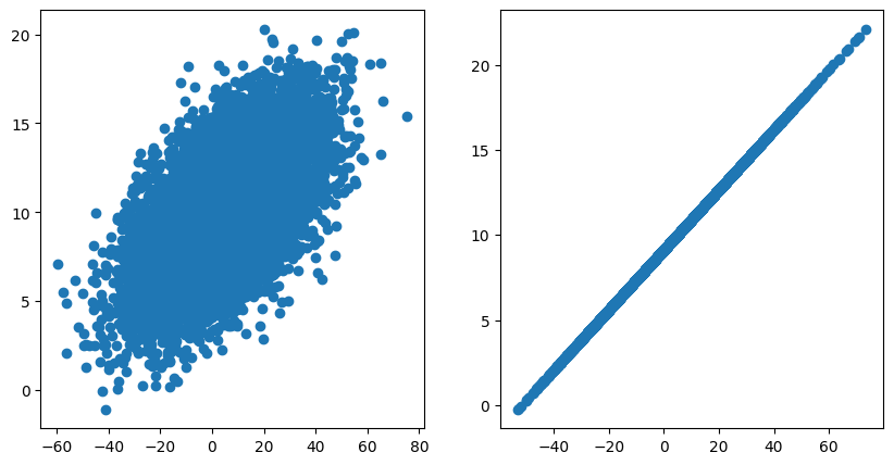
假设需要预测 ${x_i, y_i}$之间的数据关系。假设$x_i,y_i$都属于正态分布,则${x_i, y_i}$的数据关系图可以认为是两个数据的联合分布。假设${x_i, y_i}$的联合分布属于多变量高斯分布，则这个分布受制于高斯分布中的协方差矩阵。协方差矩阵描述了多个变量之间的制约关系，在离散数据点上是正定矩阵，而对于连续数据域则是协方差函数。数据关系图的不同实际上就是协方差函数的不同。因此可以把协方差定义为某些核函数，通过一步步确定核函数的表达式对数据关系进行拟合。

multivariate Gaussian：

$$p(x) = \frac{1}{(2\pi)^{D/2}|\Sigma|^{1/2}}\exp\{-\frac{1}{2}(x-u)^T\Sigma^{-1}(x-\mu)\} \\ p(x) = \frac{1}{\sqrt(2\pi)\sigma}\exp\{-\frac{(x-u)^2}{2\sigma^2}\} \quad \text{in 1-D}$$

协方差矩阵上下三角元代表变量之间的相关性，其值约大，线性相关度约大。

mu = [5, 10]

Sigma1 = array([[ 289,   30.    ],
               [  30.,   9.    ]])
Sigma2 = array([[ 289,   51.    ],
               [  51.,   9.    ]])

Kernel function ernel function:

$$<f(x), f(y)> \Rightarrow \kappa(<x,y>)$$

计算高阶内积开销很大，因此把计算高阶函数的内积转化为计算内积的高阶函数.

极端一点，若$f(\cdot)$是无限维函数，则内积$$是无法计算的，这时线内积在运用无限维函数就可以实现。

内积中的$f(x)$可以看作是把数据映射到特征空间，然后内积操作是衡量这些特征的距离。

the RBF(Radial Based Function) kernel :

$$k(x_a, x_b) = \exp{ \left( -\frac{1}{2\sigma^2} \lVert x_a - x_b \rVert^2 \right)}$$ $$k(x, x') = \sigma_f^2 \exp{ \left( -\frac{1}{2l^2} \lVert x - x' \rVert^2 \right)}$$

径向基函数radial basis functions, RBF）是一类常用的核函数, 其特点是函数值只与特征向量的二范数距离有关，并随着距离的增大而减小，且解郁0-1之间，因此是一种有效的相似度衡量方法。

Periodic kernel: model periodic functions

$$k(x_a, x_b) = \sigma^2 \exp \left(-\frac{2}{\ell^2}\sin^2 \left( \pi \frac{\lvert x_a - x_b \rvert}{p}\right) \right)$$

with:

• $\sigma^2$ the overall variance, or amplitude
• $l$ the lengthscale
• $p$ the period

Local periodic kernel:

Combining kernels by multiplication: The local periodic kernel is a multiplication of the periodic kernel with the exponentiated quadratic kernel

$$k(x_a, x_b) = \sigma^2 \exp \left(-\frac{2}{\ell_p^2}\sin^2 \left( \pi \frac{\lvert x_a - x_b \rvert}{p}\right) \right) \exp \left(-\frac{ \left\Vert x_a - x_b \right\Vert^2}{2\ell_{eq}^2}\right)$$

Kernels can be combined by adding them together.

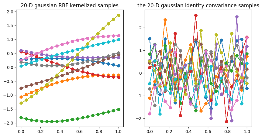
下图是 Multivariate_gaussian采样的对比。每一条线代表一个变量的采样，这种连续的曲线已经代表了变量之间的某种约束关系。右图是协方差矩阵为单位矩阵的结果，各个变量之间相互独立，因此采样点上下随机跳动。左图是添加RBF核函数作为斜方差矩阵的结果，可以看出采样点连接起来的线段比较平滑，说明变量之间已经存在制约关系，在概率的约束下有规律的波动。

当我们提高多变量的维数，采样出来的点会构成一条平滑的线，类似于数学中的函数图像。简单来说，随着变量维度的增大，这些采样出的点会越来越不需要通过线段相互连接，它们自然而然地形成一条流畅的曲线。

而当维度趋向无穷大时，可以认为该空间中的每一点都代表了一个可能的输入。这里的"输入"指的是从这个无穷维度的高斯分布中可以采样到的任何一个点或者状态。换句话说，在无限维度的情况下，高斯分布描述的是一个有着无限多参数的函数。

下图是200D的200条曲线的采样。

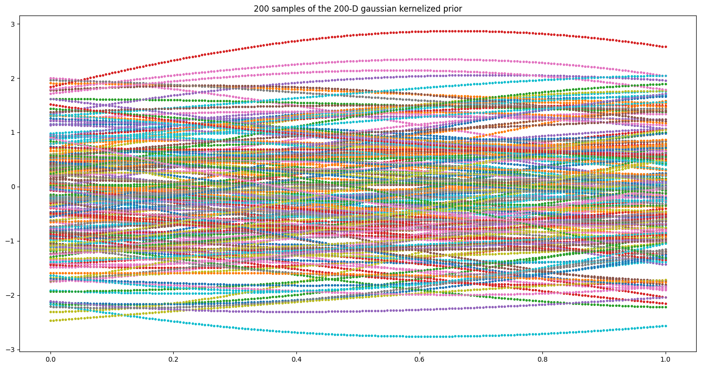
这种无穷维的分布，方便我们根据既有数据的分布决定分布概率向哪个方向集中。这样只保留所感兴趣的参数维度。这便是Gaussian Process。

A Gaussian process is a probability distribution over possible functions that fit a set of points.

Gaussian Process

Stochastic process. describe systems randomly changing over time

Gaussian processes are distributions over functions $f(x)$ as:

$$\begin{aligned}m(x) & \quad \text{mean function} \\ k(x,x')& \quad \text{positive definite covariance function} \\ f(x) &\sim \mathcal{GP}(m(x),k(x,x')) \end{aligned}$$

where for any finite subset $X ={\mathbf{x}_1 \ldots \mathbf{x}_n }$ of the domain $x$，the marginal distribution is a multivariate Gaussian distribution:

$$f(X) \sim \mathcal{N}(m(X), k(X, X))$$

This covariance function models the joint variability of the Gaussian process. choosing a specific kernel function $k$ it is possible to set prior information on this distribution.

Multivariate Gaussian Therom

$$p(x \mid \pi, \Sigma) = (2\pi)^{-k/2}|\Sigma|^{-1/2} \exp\left\{ -\frac{1}{2} (x-\mu)^{\prime}\Sigma^{-1}(x-\mu) \right\}$$

Suppose $X=(x_1,x_2)$is jointly Gaussian with parameters:

$$\boldsymbol{p(x_1,y_2)} = \mathcal{N}(\boldsymbol{\mu}, \boldsymbol{\Sigma}) \\ \boldsymbol{\mu}=\left(\begin{array}{l} \boldsymbol{\mu}_1 \\ \boldsymbol{\mu}_2 \end{array}\right), \boldsymbol{\Sigma}=\left(\begin{array}{ll} \boldsymbol{\Sigma}_{11} & \boldsymbol{\Sigma}_{12} \\ \boldsymbol{\Sigma}_{21} & \boldsymbol{\Sigma}_{22} \end{array}\right), \boldsymbol{\Lambda}=\boldsymbol{\Sigma}^{-1}=\left(\begin{array}{ll} \boldsymbol{\Lambda}_{11} & \boldsymbol{\Lambda}_{12} \\ \boldsymbol{\Lambda}_{21} & \boldsymbol{\Lambda}_{22} \end{array}\right)$$

where:

$$\begin{split} \mu_{1} & = m(X_1) \quad (n_1 \times 1) \\ \mu_{2} & = m(X_2) \quad (n_2 \times 1) \\ \Sigma_{11} & = k(X_1,X_1) \quad (n_1 \times n_1) \\ \Sigma_{22} & = k(X_2,X_2) \quad (n_2 \times n_2) \\ \Sigma_{12} & = k(X_1,X_2) = k_{21}^\top \quad (n_1 \times n_2) \end{split}$$

1. the marginal distribution of any subset of elements from a multivariate normal distribution is also normal $$\begin{array}{r} p\left(\mathbf{x}_1\right)=\mathcal{N}\left(\mathbf{x}_1|\boldsymbol{\mu}_1,\mathbf{\Sigma}_{11})\right. \\ p\left(\mathbf{x}_2\right)=\mathcal{N}\left(\mathbf{x}_2 \mid \boldsymbol{\mu}_2, \mathbf{\Sigma}_{22}\right) \end{array}$$

2. conditional distributions of a subset of the elements of a multivariate normal distribution (conditional on the remaining elements) are normal too.(the posterior conditionalis given by) $$\begin{aligned} p\left(\mathbf{x}_1 \mid \mathbf{x}_2\right) & =\mathcal{N}\left(\mathbf{x}_1 \mid \boldsymbol{\mu}_{1 \mid 2}, \boldsymbol{\Sigma}_{1 \mid 2}\right) \\ \boldsymbol{\mu}_{1 \mid 2} & =\boldsymbol{\mu}_1+\boldsymbol{\Sigma}_{12} \boldsymbol{\Sigma}_{22}^{-1}\left(\mathbf{x}_2-\boldsymbol{\mu}_2\right) \\ & =\boldsymbol{\mu}_1-\boldsymbol{\Lambda}_{11}^{-1} \boldsymbol{\Lambda}_{12}\left(\mathbf{x}_2-\boldsymbol{\mu}_2\right) \\ & =\boldsymbol{\Sigma}_{1 \mid 2}\left(\boldsymbol{\Lambda}_{11} \boldsymbol{\mu}_1-\boldsymbol{\Lambda}_{12}\left(\mathbf{x}_2-\boldsymbol{\mu}_2\right)\right) \\ \boldsymbol{\Sigma}_{1 \mid 2} & =\boldsymbol{\Sigma}_{11}-\boldsymbol{\Sigma}_{12} \boldsymbol{\Sigma}_{22}^{-1} \boldsymbol{\Sigma}_{21}=\boldsymbol{\Lambda}_{11}^{-1} \end{aligned}$$

Or:

$$p(x) = \int p(x,y) dy = \mathcal{N}(\mu_x, \Sigma_x) \\ p(x|y) = \mathcal{N}(\mu_x + \Sigma_{xy}\Sigma_y^{-1}(y-\mu_y), \Sigma_x-\Sigma{xy}\Sigma_y^{-1}\Sigma{xy}^T)$$

Noiseless GP regression

Observe a training set $\mathcal{D} = {(x_i, f_i)\, i=1:N}, f_i=f(x_i)$

GIven a test set $\mathbf{X}_$, predict the function outputs $\mathbf{f}_$

$$\left[\begin{array}{c} \mathbf{f} \\ \mathbf{f}_{*} \end{array}\right] \sim \mathcal{N} \left( \left[\begin{array}{c} \mu \\ \mu_{*} \end{array}\right], \left[ \begin{array}{cc} \mathbf{K} & \mathbf{K}_{*} \\ \mathbf{K}_{*}^T & \mathbf{K}_{**} \end{array} \right] \right)$$

where $\quad $$\begin{aligned}\mathbf{K} &= \kappa(\mathbf{X}, \mathbf{X})\\ \mathbf{K}_{*} &= \kappa(\mathbf{X}, \mathbf{X}_{*}) \\ \mathbf{K}_{**} &= \kappa(\mathbf{X}_{*}, \mathbf{X}_{*})\end{aligned}$$ $

Define the kernel:

$$k(x, x') = \sigma_f^2 \exp{ \left( -\frac{1}{2l^2} \lVert x - x' \rVert^2 \right)}$$

Predictions:

$$\begin{split} p(\mathbf{f}_* \mid \mathbf{X}_*, \mathbf{X}, f) & = \mathcal{N}(\mathbf{f}|\mathbf{\mu_{*}}, \mathbf{\Sigma_{*}}) \\ \mathbf{\mu_{*}} & = \mu(\mathbf{X}_*) + \mathbf{K}_*^T \mathbf{K}^{-1} (f - \mu_{\mathbf{X}}) \\ \mathbf{\Sigma_{*}} & = \mathbf{K}_{**} - \mathbf{K}_*^T \mathbf{K}^{-1}\mathbf{K}_* \end{split}$$

Noisy GP regression

Numerical Computation for Noisy GP regression

• input: $X$ (inputs), $\mathbf{y}$ (targets), $k$ (covariance function), $\sigma_n^2$ (noise level), $\mathbf{x}_*$ (test input)
• steps:

$$\begin{aligned}L&:=\operatorname{cholesky}(K+\sigma_n^2 I)\\ \boldsymbol{\alpha}&:=L^{\top} \backslash(L \backslash \mathbf{y}) \\ \bar{f}_*&:=\mathbf{k}_*^{\top} \boldsymbol{\alpha} \\ \mathbf{v} &:=L \backslash \mathbf{k}_* \\ \mathbb{V}[f_*] &:=k(\mathbf{x}_*, \mathbf{x}_*)-\mathbf{v}^{\top} \mathbf{v} \\ \log p(\mathbf{y} \mid X)&:=-\frac{1}{2} \mathbf{y}^{\top} \boldsymbol{\alpha}-\sum_i \log L_{i i}-\frac{n}{2} \log 2 \pi \end{aligned}$$

• return: $\bar{f}_$ (mean), $\mathbb{V}[f_]$ (variance), $\log p(\mathbf{y} \mid X)$ (log marginal likelihood)

Tuning hyperparameters

$$\begin{aligned}\hat{\theta} &= \underset{\theta}{\text{argmax}} \left( p(\mathbf{y} \mid X, \theta) \right) \\ p(\mathbf{y} \mid \mu, \Sigma) &= \frac{1}{\sqrt{(2\pi)^d \lvert\Sigma\rvert}} \exp{ \left( -\frac{1}{2}(\mathbf{y} - \mu)^{\top} \Sigma^{-1} (\mathbf{y} - \mu) \right)} \\ p(\mathbf{y} \mid X, \theta) &= \frac{1}{\sqrt{(2\pi)^d \lvert \Sigma_{\theta} \rvert}} \exp{ \left( -\frac{1}{2}(\mathbf{y} - \mu_{\theta})^\top \Sigma_{\theta}^{-1} (\mathbf{y} - \mu_{\theta}) \right)} \\ \log{p(\mathbf{y} \mid X, \theta)} &= -\frac{1}{2}(\mathbf{y} - \mu_{\theta})^\top \Sigma_{\theta}^{-1} (\mathbf{y} - \mu_{\theta}) - \frac{1}{2} \log{\lvert \Sigma_{\theta} \rvert} - \frac{d}{2} \log{2 \pi} \\ \hat{\theta} &= \underset{\theta}{\text{argmax}} \left( p(\mathbf{y} \mid X, \theta) \right) = \underset{\theta}{\text{argmin}} { \;-\log{ p(\mathbf{y} \mid X, \theta)}} \end{aligned}$$

\slug \slug \slug \slug \slug \slug \slug \slug \slug

Gaussian Process Motion Planning

continuous-time trajectory as a sample from a Gaussian process (GP) generated by a linear time-varying stochastic differential equation

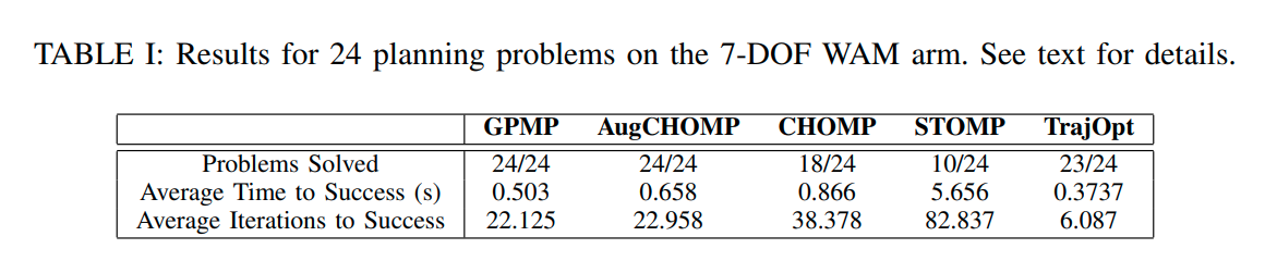
Experiment

(trajopt's efficiency is the best)

Ref

• PAPER
  • Gaussian Processes for Regression:A Quick Introduction
  • 2016 icra - Gaussian process motion planning
  • 2016 rss - Motion Planning as Probabilistic Inference using Gaussian Processes and Factor Graphs
  • 2018 Continuous time Gaussian process motion planning via probabilistic inference
  • 2012 Optimal trajectories for time-critical street scenarios using discretized terminal manifolds
• PROJECT
  • gpmp2: Gaussian Process Motion Planner 2