04-GLM

残差分布

采样数据$(X,Y)$, 对任意一个自变量$y^i$,有一个对应的模型预测值$\hat{y}^i=h(x^i, \theta)$. 从概率的角度来看，模型估计出来的不是一个值，事实上是一个分布$P(\hat{y}^i|x^i,\theta)$, 并且对每一个自变量$y^i$都有一个分布。而所谓的预测值是该分布的期望$\hat{y}^i=E(\hat{h}^i)$. 残差指的是在分布$P(\hat{h}^i|x^i,\theta)$下，采样得到的数据与期望的偏差$y^i-E(\hat{h}^i)=y^i-\hat{y}^i$, 当然最后的表达式很直接，就是真实值与预测值之间的差。

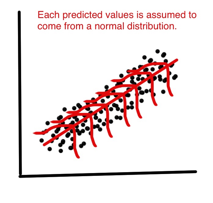
残差的分布是指在分布$P(\hat{h}^i|x^i,\theta)$下偏差的分布。需要注意的是这里的分布都是针对当前单个采样点$y_i$来说的，即我们假设该采样点$y_i$虽然只有一条数据，但它事实上来自于一个分布。如下图所示，每一个预测点附近都产生了一个分布,通过这个分布采样了一个$y^i$. 当然单个采样点无法绘制出整个分布图，但可以通过取一段区间里面的数值来重现这种分布。或者根据大数定理，可以通过对所有采样点的残差分布来近似当前采样点的残差分布(?).

把误差(残差？)细分为两大类，一类是模型由于估计不足造成的误差，一类是由于采样造成的不可消除误差, 即真实值认为是从从一个分布中采样的数据，而预测值是分布的期望，这两者之间的残差不可消除。如果一个模型达到最优，则误差仅剩不可消除误差。根据大数定理，在大样本统计下，该误差满足高斯分布$\epsilon=P(y^i-\hat{y}^i)\sim N(0, \sigma^{2}) $, 由于$\epsilon=y^i-\hat{y}^i$, 并且对于分布$P(y^i|x^i,\theta)$,$\hat{y}^i=E(\hat{h}^i)$是一个常数， 根据高斯分布的性质则$y^i\sim N(\hat{y}^i, \sigma^{2}) $, 即隐变量满足高斯分布：

$$ $$\begin{align}P(y^i)&=\frac{1}{\sqrt{2 \pi} \sigma} \exp \left(-\frac{(y^i-\hat{y}^i)^{2}}{2 \sigma^{2}}\right) \\ \text{似然函数：}\quad L(\theta)&=\prod^t_{i=1} P(y^i-\hat{y}^i) \\ \text{最大似然估计：}\quad \max_{\theta} \log(L)&=\sum (\log{\frac{1}{\sqrt{2 \pi} \sigma}} -\frac{(y^i-\hat{y}^i)^{2}}{2 \sigma^{2}}) \\ \Downarrow & \quad \text{$\sigma$ 为常数，故略去。并且假设不同的采样点有相同的$sigma$}\\ \text{损失函数：}\quad \min_{\theta} -\log(L)&=\sum(y^i-\hat{y}^i)^{2}\end{align}$$ $$

上式中均方损失函数的推导过程事实上就是线性回归采用该损失函数的原因。在这个过程中有一个关键的假设就是残差分布满足高斯分布。如果把线性回归拓展成多项式回归，即数据在多项式模型周围也应该呈0均值高斯分布，则通过推导，多项式回归的最大似然函数也是均方损失。这也是比较直觉的一个表达式：对于大部分模型拟合，均方损失确实能反映出拟合情况，这事因为根据大数定律，在数据量较大的情况下误差满足高斯分布。

虽然残差满足高斯分布的假设适用于多项式拟合的情况，但是对于分类任务会有所不同。通过观察发现高斯分布更适合于连续值预测的情况，而对于分类任务中的离散值，比如二分类，则其分布更应该假设为Bernoulli分布。

通过以上讨论可知，残差分布(因变量分布)通过最大似然估计决定了用什么样的损失函数，这个可以认为是数据的局部分布。而数据整体的分布决定了该用什么模型，这叫做数据的整体分布。

The generalized linear model (GLM, 广义线性模型) is a flexible generalization of ordinary linear regression.把自变量的线性预测函数当作因变量的估计值。The target variable y is also called response variable in GLM.

线性回归和逻辑回归

现在来回答为什么线性回归使用均方损失。对于一个具体的任务可以有很多个模型去拟合。而如果我们选择了一个模型，则有很多种损失函数选择。线性回归也有适合于该模型的具体任务。如果假设在数据中找到一个线性模型，并且采样点在该模型周围（残差）呈0均值高斯分布，则由最大似然估计得出其损失函数为均方损失。因此线性回归使用均方损失的原因可以归结为我们先假定了数据在一个线性模型周围呈0均值高斯分布。而如果这个任务确实适合线性模型拟合，则这种假设通常也是成立的。如果一个任务不适合线性模型，则通过线性模型拟合的残差也不会呈高斯分布，即选错了模型。这一过程可以总结为：先做了一个假设，根据假设求得了一个模型，并反证得出该假设是成立的。总之，当我们采用一个模型的时候，总是假设这个模型就是该任务的最优模型来求解的。

对于逻辑回归，其因变量假设服从Bernoulli分布：

$$p(y|x;\theta)=(h_\theta(x))^y(1-h_\theta(x))^{1-y} \\$$

$$\begin{align}L(\theta)&=\prod_{i=1}^mp(y^{(i)}|x{(i)};\theta)\\&=\prod_{i=1}^m(h_\theta(x^{(i)}))^{y^{(i)}}(1-h_\theta(x^{(i)}))^{1-y^{(i)}}\end{align} \\$$

$$l(\theta)=logL(\theta)=\sum_{i=1}^my^{(i)}logh(x^{(i)})+(1-y^{(i)})log(1-h(x^{(i)})) \\$$

the exponential family

the prototype:

$$\begin{equation}p(y; \eta)=b(y)exp(\eta^TT(y)-a(\eta))\end{equation} \\$$

Here, $\eta$ is called the natural parameter(or canonical parameter); $T(y)$ is the sufficient statistic, which is often the case: $T(y)=y$; $a(\eta)$ is log partial function. The quantity $e^{-a(\eta)}$ essentially plays the role of a normalization constant, that makes sure the distribution $p(y;\eta)$ sums/integrates over y to 1. A fixed choice of T,a and b defines a family of destributions that is parameterized by $\eta$;we then get different distributions within this family.

We now show that some common distributions belong to the exponential family.

Gaussian distributions:

$$\begin{align} p(y)&=\frac{1}{\sqrt{2\pi\sigma}}exp(-\frac{(y-\mu)^2}{2\sigma^2})\\&= \frac{1}{\sqrt{2\pi\sigma}}exp(-\frac{y^2-2y\mu^2+\mu^2}{2\sigma^2})\\&=\frac{1}{\sqrt{2\pi\sigma}}exp(-\frac{y^2}{2\sigma^2})\cdot exp(\frac{\mu}{\sigma^2}\cdot y-\frac{y^2}{2\sigma^2})\end{align}$$

Bernoulli distribution:

$$\begin{align}p(y)&=\phi^y(1-\phi)^{1-y}\\&=exp(ylog\phi+(1-y)log(1-\phi))\\&=exp((log(\frac{\phi}{1-\phi}))y+log(1-\phi)) \end{align}$$

Thus, the natural parameter is given by $\eta=log(\phi/(1-\phi))$. If we invert this definition for $\eta$ by solving for $\phi$, we obtain $\phi=\frac{1}{1+e^{-\eta}}$. This is the familiar sigmoid function. Actually, the ordinary least squares(最小二乘法) is based on Gaussian distribution, and logistic regression on Bernoulli distribution.

constructing GLM

three assumptions:

• $y\vert x;\theta ~ExponentialFamily(\eta)$. I.e., given x and $\theta$, the distribution of y follows some exponential family distribution, with parameter $\eta$.
• $h(x)=E[T(y)|x]$.
• The natural parameter $\eta$ and the inputs $x$ are related linearly: $\eta=\theta^Tx$, which might be better thought of as a "design choice".

softmax regression

Consider a classification problem in which the response variable $y$ can take any one of k values, so $y\in {1,2,...,k}$. We use k parameters $\phi_1, \cdots,\phi_k$ specifying the probability of each of $y$. we will instead pa- rameterize the multinomial with only $k − 1$ parameters, $\phi_1, \cdots,\phi_{k-1}$, and $p(y=k)=1-\sum_{i=1}^{k-1}\phi_i$.

To express the multinominl as an exponential family distribution, we introduce one more very useful piece of notation. $[1{true}=1,1{false}=0 ]$ and define $[(T(y))_i=1{y=i}]$. Then we have that $E[(T(y))_i]=p(y=i)=\phi_i$. so:

$$\begin{align} p(y;\phi)&=\phi_1^{(T(y))_1}\cdots\phi_{k}^{\sum_{i=1}^{k-1}(T(y))_{i}}\\&=exp((T(y))_ilog(\phi_i)+\cdots+(1-\sum_{i=1}^{k-1}(T(y))_i)log(\phi_k))\\&=exp((T(y))_ilog(\frac{\phi_i}{\phi_k})+\cdots+log(\phi_k))\\&=b(y)exp(\eta^TT(y)-a(\eta)) \end{align} \\$$

where:

$$\eta=\begin{bmatrix} log(\phi_1/\phi_k)\\\cdots\\log(\phi_1/\phi_k) \end{bmatrix}\\a(\eta)=-log(\phi_k) \\$$

$$T(i)=\begin{bmatrix}0\\0\\\cdots\\1\\\cdots\\0\end{bmatrix} , i-th\quad is 1\\$$

the link function is given (for i=1,...,k) by:

$$\eta_i=log\frac{\phi_i}{\phi_k} \\$$

And:

$$\phi_k\sum_{i=1}^ke^{\eta_i}=\sum_{i=1}^{k}\phi_i=1\\\phi_i=\frac{e^{\eta_i}}{\sum_{j=1}^k e^{\eta_j}} \\$$

By assumption 3: $\eta=\theta^Tx$:

$$p(y=i|x;\theta)=\phi_i=\frac{e^{\eta_i}}{\sum_{j=1}^k e^{\eta_j}}=\frac{e^{\theta_j^T x}}{\sum_{j=1}^k e^{\theta_j^T x}} \\$$

Our hypothesis will output:

$$\begin{align} h_\theta(x)&=E[T(y)|x]\\&=E\begin{bmatrix} 1\{y=1\}\\\cdots\\1\{y=k-1\}\end{bmatrix}\\&=\begin{bmatrix} \phi_1\\\cdots\\\phi_{k-1}\end{bmatrix} \\&=\begin{bmatrix} \frac{e^{\theta_1^T x}}{\sum_{j=1}^k e^{\theta_j^T x}} \\\cdots\\\frac{e^{\theta_{k-1}^T x}}{\sum_{j=1}^k e^{\theta_j^T x}} \end{bmatrix}\end{align} \\$$

Our hypothesis will output the estimates probability for $p(y=i|x;\theta)$,[$p(y=k)=1-\sum_{i=1}^{k-1}p(y=i)$].The log-likelihood is:

$$l(\theta)=\sum_{i=1}^{m}log\prod_{i=1}^k(\frac{e^{\theta_l^T x^{(i)}}}{\sum_{j=1}^k e^{\theta_j^T x^{(i)}}})^{1\{y^{(i)}=l\}} \\$$

ref

• 从线性模型到广义线性模型（1）——模型假设